For both FIFO Conveyors (see FIFO Conveyor Computation) and Traditional Conveyors (see Traditional Conveyor Computation) material can be set to spread across the existing conveyor content rather than enter at the beginning of the conveyor. This is very useful when the material coming into the conveyor is not all of the same age. For example, if the conveyor is for people age 30-34, then immigration would be expected to include people with all ages in the group and not only people age 30.
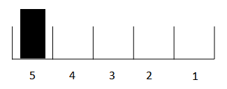
To understand how spreading works consider the case of a conveyor with a transit time of 5 hours for a DT of 1. In this case there are 5 spots that material could be put in:

Where the position marked 5 will be released in 5 hours, 4 in 4 hours, 3 in 3 hours, 2 in 2 hours, and the one marked 1 will be released in 1 hour (the next DT). Normally, new material is all deposited in 5:

In this case that everything will wait 5 hours till it flows out. This is the normal conveyor process.
Rather than adding all the material at position 5, we could spread the material out evenly:

In this case, 1/5th of the material would come out in an hour, one fifth in two hours and so on.
There are, in addition to putting all the material at the beginning of the conveyer, four ways to spread the material: evenly, as in the above example, proportional to what is already there, based on where the material came from (a special case), and using a graphical to define a profile. These three choices are set on the flow.
Flow spreading is set as an option on the inflow to the conveyor:

The first choice (At Beginning) is the default and it is the standard way that a conveyor behaves. The remaining choices are described below.
Note The fifth choice (Based on Source) is only available if the flow is a conveyor leakage.
This is the default:

Material added will be released after the transit time.
The same amount of material goes in all positions on the conveyor.

Material will be divided up evenly with the same amount coming off the conveyor every DT. If a pulse input were to be added, the outflow would be constant until the material was exhausted.
This selection is useful when you want new material to mix with existing material for the purposes of dispatching it. For example, material pulled off an assembly line for rework might be put back on the assembly line in its partially completed state.
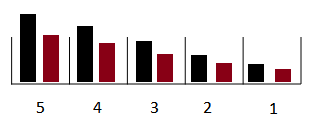
Material is added proportional to what is already on the conveyor.

The black bar shows what was already in the conveyor, and the brown bar what is being added. The amount added at each position is the same portion of the amount of material already there. The total amount added (sum of the brown bars) is the value of the flow.
This selection is useful when you would expected new additions (for example, those that might occur because of immigration) to be distributed the same as the existing population.
When this option is selected there will be an editing box to enter the name of either a graphical function or a 1 dimensional array slice:

Type in the name, or select if from the input list (you will need to draw a connector from this input to the flow). In this case material will be distributed based on the shape of the graphical or the array entries. For example:
Usting delay_array[*] as the distribution table with:
delay_array[1] = 2
delay_array[2] = 3
delay_array[3] = 4
delay_array[4] = 3
delay_array[5] = 1
Or using delay_graphical as the distirbution table with:
delay_graphical = GRAPH(0+0)
Points: (0.000, 2.0), (1.000, 3.0), (2.000, 4.0), (3.000, 3.0), (4.000, 1.0), (5.000, 1.0) {GF DISCRETE}
Would result in:

Here more material is delayed 3, and very little 1. The average delay time, therefore, is less than 5. Distribution table is automatically normalized so that it is effectively a probability density function. The last value comes out soonest, the first last. To get the same effect from a graphical there needs to be an extra point with the last point repeated and the graphical marked as discrete.
If you want to set up a conveyor to have a target average transit time then you make sure the profile is defined on [0,1], and use the equations:
delay_profile ((0,0.5),(0.5,1),(0.8,0.1),(1.0,0))
average_delay = 8
maximum_delay=INIT(average_delay/LOOKUPMEAN(delay_profile,1)
These equations will give an average delay of 8, with the maximum bigger than 8. It is critical that the graphical be on the range [0,1] for this to work.
Working with array slices this would become:
delay_array[*]=0.5,1,2,1,0.1
t_normalized[*]=0.1,0.3,0.5,0.7,0.9 {ddim/SIZE(ddim) - 1/SIZE(ddim)/2 would be generic }
average_delay = 8
maximum_delay = average_delay/(SUM(delay_array[*]*t_normalized[*])/SUM(delay_array[*])
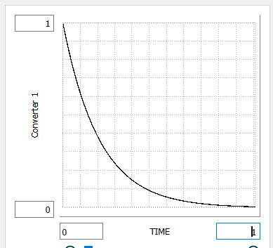
The graphical used need not be discrete, it can be interpolated to give finer granularity. For example, using a profile that is (approximately) a negative exponential:

Will give you a conveyor that behaves approximately the same as a normal stock where the outflow is just stock/average_delay_time. The profile thus gives you the ability to have different types of delays including the approximation of nth order delays.
This option places material on the conveyor based on the amount pulled from the corresponding position in an upstream conveyor. It is only available when a conveyor leakage is being used as the inflow to another conveyor.


This choice is most useful when the two conveyors have the same transit time, and works best when the leakage is exponential (with 0 to 100 leak zone). It basically transfers the leakage onto the next conveyor. It is very useful when you have aging material in the conveyors, and that material can transition to another state (as in the case of disease onset and progression in an aging population).
Normally the actual leakage at each position is used (though sometimes this is not possible and then an amount proportional to the material at each position is used). In the case of exponential leakage these two are the same.
If the two conveyors have the same (constant) transit time and the leakage is exponential, then no delay is introduced. This allows you to maintain the integrity of an aging chain. Always use exponential leakage if you want to capture simultaneous aging and progression in a population.
Note If leakages are linear, not on a 0 to 100 leak zone, or if transit times are variable or differ between the 2 conveyors, then a delay of approximately DT is effectively introduced between the source and destination conveyors.
Under some circumstances, especially if leakage rates depend on the stock they are leaking from, it may not be possible to make everything line up and a delay of DT will also be introduced.
When inflows are spread, linear leak fractions will be applied only for the duration the material is in the conveyor. With an inflow that is spread evenly over the conveyor this means a leak fraction of 0.5 will only result in approximately 25% of the material leaking. If you want the leak fraction to apply to all of the incoming material, independent of how long it says in the conveyor, then select the options "Leak same fraction for all durations" in the Equation Tab for the leakage.