This section describes the following builtins:
Present value (pv), future value (fv), periodic payment (pmt), number of periods (nper), and interest rate per period (rate) are standard financial parameters in cash flow problems involving constant payments. The FV, PMT, and PV builtins calculate future value, periodic payment, and present value based upon the values of the other financial parameters.
Use the following cash flow conventions in depicting PV, FV, and PMT: cash received is represented by a positive number, cash paid out is represented by a negative number. See the example below for an illustration. Note that rate and nper must refer to the same period. For example, if nper is the number of months, then rate must be the effective monthly interest rate. Finally, for each of the financial builtins, the first payment is assumed to occur at the end of the first period.
The software uses the following equations to solve for one financial argument in terms of the others:
pv * (1 + rate)nper + (pmt / rate) * ((1 + rate)nper -1) + fv = 0
(for rate <> 0)
pv + pmt * nper + fv = 0
(for rate = 0)
Example:
You received an automobile loan of $10,000, at an effective monthly interest rate of 1%. You must repay the loan in 36 monthly payments made at the end of each month. What are your monthly payments?
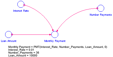
Your structural diagram, and the corresponding equations, are shown in the following figure.
The software returns the value for Monthly Payment as -332.14, indicating that the payment is an expense.

The IRR function returns the interest rate that would make the net present value of a stream of payments 0. This is often used as a measure of the value of a project or product. The stream argument needs to include both negative and positive values - for example investment and receipts. The optional missing argument will be used initially, and any other time that there is no solution that can be found (for example is all values are positive). The stream argument can represent either payments or receipts (this is because the IRR of x and -x will be the same).
Examples:
Internal_Rate_Of_Return_Receipts = IRR(net_receipts), where net receipts is -100 in year 1 (an investment), then 10 in each of the next 19 years (with DT of 1 year) will return 0.074 (7.4%). If the model runs longer, the value will eventually converge on 0.1 (10%). In year 0 it will return NaN, then negative numbers increasing to the 0.074 value.
Internal_Rate_Of_Return_Borrowing = IRR(net_borrowing,-10), where net payments is 100 in year 1 (the loan), then -10 in each of the next 19 years (repayment) will return 0.074 (7.4%). In year 0 it will return -10, then follow the same pattern as the first example.
Internal_Rate_Of_Return_Extreme = IRR(two_period,0), where two period is -100 in year 1 and 50 in year two will return -0.5, indicating that future values are not discounted, but inflated.
Note If you change DT from 1 to a smaller number the above examples still work (using one value for each DT in the first year, then another in successive years) but the numeric results will be slightly different.
When the input to the IRR function follows the above pattern - one or more values of one sign, followed by a sequence with the opposite sign, there will be a unique solution giving a 0 NPV. If, however, the first argument moves back and forth between positive and negative, there may be multiple (or no) solutions. The software will try to find the smallest (in absolute value) solution possible, and return the second argument or NaN if no solution is found. The initial value returned is always the second argument (or Nan if only 1 argument is used). The next several returned values are often negative. Since it is the final value that is typically of interest you can use a formulation such as:
IF TIME = STOPTIME THEN IRR(stream) ELSE 0
so that only values of interest are displayed.
The NPV function calculates the net present value of a stream of input, using a discount rate of rate; rate refers to the effective per-period discount rate for your model simulation. The value returned by NPV is the present value (at the outset of your simulation run) of the stream of inputs from model start time to a given simulation time. You may specify an optional initial value initialfor the calculation; otherwise, the initial value of input serves as the initial value.
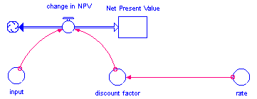
The NPV function, when used in a converter, will produce the same results as the stock in the structure and equations shown below. The discount factor is normalized to the Time Specs setting for start time, so that the initial condition of the denominator evaluates to a value of 1.

change_in_NPV = input * discount_factor
discount_factor = 1/(1 + rate)^(TIME - STARTTIME + DT)
input = constant or variable
rate = constant or variable
INIT Net_Present_Value = constant
Examples:
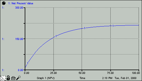
Net_Present_Value = NPV(10, .05) generates the pattern shown in the following graph. The values for Net Present Value represent the present value - at time 0 - of the constant stream of benefits, given the effective per-period discount rate of 5%.
