Two types of situations require special care when choosing the value for DT:
If you understand these two types of situations, and you also make a practice of running the "1/2 test", you should have minimal difficulties with DT.
Both situations are described in more detail below.
Artifactual delays result from the fundamental conceptual distinction between stocks and flows. Stocks exist at a point in time. Flows exist between points in time. As such, the two can't co-exist at the same instant in time.
Look at the first table of values in DT examples. Notice that Cash is 0 at TIME = 0. The first value of income that appears in the table is $25. It appears at TIME = 0. But it really exists between TIME = 0 and TIME = 0.25. This is why Cash doesn't equal $25 until TIME = 0.25. It takes one DT to integrate (in a mathematical sense) the value of the flow to yield a new value for the stock. There's no way to get around this integration delay. And, conceptually, it's real. It reflects the inevitable delay that exists between the time a decision to take some action is made, and the time it takes for the resulting action to make itself felt in one or more accumulations. For example, if you decide to eat that cookie beckoning to you from the plate, it will take an "instant" before you can seize it. You can't decide to seize and seize in exactly the same instant. This "instant" is the software's artifactual delay.
As long as DT is defined as a relatively small value, artifactual delays are usually insignificant. It's usually only when DT becomes too large that such delays become a problem. We say "usually" because, in some cases (even with a small DT), small integration delays can add up. In these cases, lots of little delays make one big delay, and that big delay can distort the model's dynamics. Let's look at a case in which this distortion occurs.
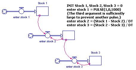
Suppose that we have three stocks arranged such that the first transmits information about its magnitude to the inflow that feeds the second. The second, in turn, transmits similar information to the inflow that feeds the third. A diagram of this arrangement appears below.

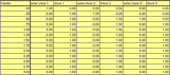
The inflow to "Stock 1", "enter stock 1", is defined with the PULSE Builtin function. The PULSE fires off a 1.0 at TIME = 0. Once the 1.0 arrives in "Stock 1", this becomes a signal to fire a 1.0 into "Stock 2". Once "Stock 2" is "loaded," it triggers a 1.0 to flow through "enter stock 3". We'll simulate this system twice, once with DT = 0.25 and once with DT = 1.0. When we do, we get the results shown in the following tables.
DT = 0.25
DT = 1.0

Note: In these tables, stocks are reported with beginning balances and flows use summed reporting.
Tracing the initial pulse through the system, we see that, with DT = 0.25, the pulse doesn't arrive in Stock 3 until TIME = 0.75, three DTs after it's fired. The delay in arriving is due to the implicit one DT "perception lag" built into any such stock-to-flow-to-stock connection. Since there are two such connections in this system, we should expect to wait two DTs for the message to complete its journey. The third DT lag is contributed by the integration delay between enter stock 1 and Stock 1. These artifactual delays become a bit more of an issue when DT is 1.0 or larger. In the case of DT=1.0, a three DT lag means three months.
If you have sequences in which one stock is generating the input to a flow that feeds a second stock (and so on), you'll need to use care in selecting a value for DT. In these instances, you'll probably want to make DT less than 1.0 to avoid the cumulative effect of such perception lags.
The second area requiring special care in the choice of DT arises when your model generates a dynamic pattern of behavior caused by the way the software is performing its calculations. What happens in these cases is that, because the value of DT is too big, the flow volumes remain too big, and "pathological" results are generated. In effect, the flow overwhelms the stock to which it's attached.
To illustrate how "overwhelming" can come about, let's return to the first table of values in DT examples. In that example, we had a stock of "Cash" being fed by a flow of "income". Adding an outflow yields the following diagram:

In this model, "Cash" is drained by "spending". The flow "spending" is defined as a graphical function that takes "Cash" as its input. The graphical function used to specify spending is shown below.
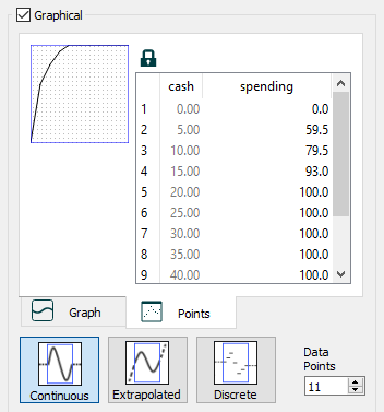
The initial value of the "Cash" stock is $100, and "income" remains constant at $90/month. DT is set at 1.0.
The following graph presents the results of a simulation of this model.
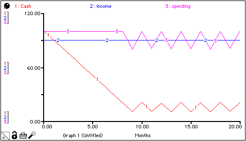
The results indicate that "Cash" will drain down for awhile, and then "saw-tooth" about a steady-state value, which appears to be somewhere around $12 to $15. Spending remains constant at $100 per month until "Cash" dips below $20 (see the graphical function, above), then it too, begins to saw-tooth.
Whenever you see such a saw-tooth pattern, always run the "1/2 test". The results of this test for this model appear below.
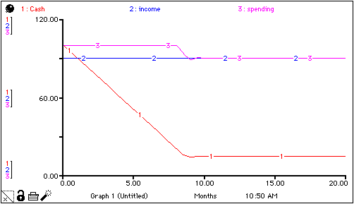
As you can see, only the barest hint of a saw-tooth pattern remains. This "hint" would completely disappear if we cut DT in half once again. The pattern would disappear because it's being generated as an artifact of a calculation problem, not by the interplay of the relationships in the system!
Just what is this calculation problem? As soon as "Cash" dips below $20, spending begins to decline. What should happen is that, as spending falls, "Cash" should begin to decline at a decreasing rate. This is because the rate at which "Cash" is declining is simply equal to the difference between income and spending. And, since spending is falling (and income is constant), then the difference between the two is getting smaller. As such, "Cash" should decline more and more slowly as spending gets closer and closer to income. "Cash", therefore, should gradually approach a value where it will generate a value for spending that's exactly equal to income (that is, $90). This is essentially what happens when DT is cranked down to 0.5, and exactly what happens for values of DT less than 0.5. But it's not what happens when DT is 1.0.
When DT is "too big", the cut back in spending doesn't occur soon enough. In fact, spending remains too high for one DT. This causes "Cash" to drop below its steady-state value (the value at which spending will decline to just equal income). Because "Cash" falls below its steady-state value, it generates a value of spending that's less than the value of income. With income in excess of spending, "Cash" increases. But, once again, because DT is too big, the rebound carries "Cash" past its steady-state value. This means that spending is again in excess of income. So, once again "Cash" must fall. And, we're back into the cycle. When DT is reduced, "Cash" is able to directly home in on its steady-state value without overshooting or undershooting. This is because with a smaller DT, the incremental changes in spending are smaller (since calculated flow values are multiplied by DT). As such, spending can gradually approach income, rather than "hopping over" it.
It may help you to see what's going on in the model to generate values for "Cash", "income", and "spending" in a table for different values of DT. It will also be useful to create a graph of "Cash". For small values of DT, you'll see it smoothly home right in on its steady-state value with no overshoot whatsoever.
Picking a value for DT that's too big can lead to all sorts of mayhem. This is particularly true when a stock (with the Non-negative check box unselected) has a bi-directional flow whose value is determined as some function of the stock. What happens in this case is that, when the biflow's outflow volume "overwhelms" the stock, the stock goes negative. Then, because the flow depends on the stock, it too goes negative. But a negative outflow is equivalent to an inflow, so, the flow reverses, putting stuff back into the stock. This enables the outflow to be positive once more, re-initiating the cycle. Once again, the manifestation of the problem is a saw-tooth oscillation. In this case, the stock oscillates between a positive and negative value (and sometimes the amplitude of the oscillation will expand).
The bottom line here is that if you see a saw tooth oscillation (or any oscillation, for that matter), it's always a good idea to run the "1/2 test". Make sure that the oscillation is real, and not an artifact of your choice of value for DT. Real oscillations will persist even with the tiniest values for DT.
Practically speaking, if you keep DT at, or below, 0.25, it's unlikely that you'll ever encounter any of the problems discussed here. However, it's important that you be aware of what DT is doing in your models. This will keep you from being puzzled when strange behaviors appear in your model results. It'll also equip you for correcting such strangeness if it does appear. If you encounter unexpected delays in your models, or you see a puzzling behavior pattern (particularly, a saw tooth oscillation), check DT. Cut it in half and re-run your model. If the results persist, try cutting it in half one more time. If the results continue to persist, it's very likely that the behavior you're seeing is real. If the behavior disappears, it was a calculation artifact.